Road to Efficient LLMs 1: LoRA

Given the rapid advancements in large language models (LLMs) like the recent launch of Llama 2 and research focusing on parameter efficiency, hallucination reduction, and accelerated inference, we’re seeing the gap close between open-source models and commercial solutions like ChatGPT. Companies today often don’t require a Jack-of-all-trades language model capable of solving complex mathematical equations; they’re looking an LLM that excel at specific tasks relevant to their domain. Fine-tuning a large language model on a custom dataset is increasingly becoming a practical and efficient choice. That’s why I’m launching a series called ‘Road to Efficient LLMs,’ where I’ll explore the latest techniques for fine-tuning and optimizing these powerful models for real-world applications. Note: While you can certainly fine-tune models like GPT-3.5, having your own large language model offers greater flexibility and can be more cost-effective for experimentation.

Introduction

Large Language Models (LLMs) are undoubtedly powerful, thanks to their extensive training on massive amount of datasets. However, their generalized knowledge isn’t always sufficient for specialized tasks that demand high accuracy. The good news is, you don’t have to start from scratch to make them domain-specific experts. A few epochs of focused training, known as fine-tuning, can do the trick. Yet, the enormous size of these models (Currently,largest open-source model to is Falcon with 180 billions parameters), makes fine-tuning a daunting task on consumer-grade GPUs. Today, we’ll explore one of the solution to this challenge: LoRA: Low-Rank Adaptation of Large Language Models. Note: While our focus is on LLMs, it’s worth noting that this method can be applied to any neural network with weight matrices.

Background concepts

Before delving into the explanation of LoRA, it’s crucial to grasp the concepts of matrix rank and decomposition. Simply put, the rank of a matrix is the number of linearly independent rows or columns, or in other words, number of unique rows (that are not made from other rows, same concept applied to column as well). To demystify this definition, consider a straightforward example.

Imagine we have a Matrix $X$ of size $2*3$,

\[\left[\begin{array}{lll} 1 & 2 & 3 \\ 3 & 6 & 9 \end{array}\right]\]

Upon examination, it’s evident that the second row is thrice the first, which implies that Matrix $X$ has only one unique row, rendering it a rank 1 matrix. In order word, it only have one unique row or rank 1. Consequently, $X$ can be decomposed into two smaller matrices, $A$ and $B$, with dimensions $2×1$ and $1×3$, respectively:

\[\left[\begin{array}{lll} 1 \\ 3 \end{array}\right] * \left[\begin{array}{lll} 1 & 2 & 3 \\ \end{array}\right] = \left[\begin{array}{lll} 1 & 2 & 3 \\ 3 & 6 & 9 \end{array}\right]\]

Now, instead of having a full-rank matrix $X$, we could represent it with two low-rank matrices matrix $A$ and $B$ which closely resemble the original full-rank matrix $X$. As another example, consider a matrix of size 1000 * 1000, We could approximate it with two matrices of sizes $1000 * 100$ and $100 * 1000$, where 100 is the rank. This approach reduces the number of elements in the matrix from 1,000,000 -> 100,000+100,000. More formally, for a matrix $W \in \mathbb{R}^{d \times k}$, we could decompose it into two matrix $B \in \mathbb{R}^{d \times r}$ and $A \in \mathbb{R}^{r \times k}$, where $r \ll \min (d, k)$. Note: The example above can be applied to columns as well.

LoRA

Concepts

LoRA is build on top of the hypothesis that state:

..the change in weights during model adaptation also has a low “intrinsic rank”

This implies that updates to the original weight matrices can be represented as low-rank matrices. Recap the previous section, suppose $W \in \mathbb{R}^{1000 \times 1000}$ represents the updates to the original weight matrix. This matrix could be approximated by two other matrices with $B \in \mathbb{R}^{1000 \times 10}$ and $A \in \mathbb{R}^{10 \times 1000}$. Training matrices $A$ and $B$ can therefore approximate the weights derived from full fine-tuning. The forward pass of a model (assuming it is a single layer) can be formally expressed with the following equation:

\[h=W_0 x+\Delta W x=W_0 x+B A x\]

where $h$ is the output of current layer, $W_0$ is the original pre-trained weights (frozen), $\Delta W$ is the update of original weights, $BA$ is the low-rank weight and $x$ is the input.

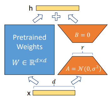
To better understand, refer to the visuals provided above. Given input $X \in \mathbb{R}^{d}$, the left segment (depicted in blue) represents the original pre-trained weights $W \in \mathbb{R}^{d \times d}$,while the right segment (in orange) showcases two low-rank matrices $A \in \mathbb{R}^{d \times r}$ and $B \in \mathbb{R}^{r \times d}$. During inference, we could add the original weights and matrix $BA$ to get output $h$ as describe in previous equation. Note: They use a random Gaussian initialization for A and zero for B, so ∆W = BA is zero at the beginning of training.

Advantage of LoRA

Memory and Storage Efficiency: Since updates aren’t performed on the original weight matrices, only the gradients of the low-rank weight matrices need to be stored. As such, the gradients of the pre-trained, frozen weights are neither required nor calculated. This approach is particularly efficient when dealing with low-rank matrices, resulting in significant reductions in memory and storage requirements. For a more technical explanation, please refer the discussion here.
Able to switch between task. Consider a scenario involving a model with 170 billion parameters intended for use on multiple downstream tasks. Storing multiple models of this size is not only costly but also inefficient. However, with fine-tuned adapters designated for each task, switching between tasks can be accomplished with minimal memory overhead. We could simply substract $W$ with $BA$ to recover the original weights and adding a different $B^{\prime} A^{\prime}$.

Implementation

Pretrained Model

As LoRA is primarily utilized for fine-tuning large models, we will begin by implementing a simplified model that will act as our “pre-trained model”. For the sake of simplicity, this model will be trained using the CIFAR-10 dataset.

class CifarModel(nn.Module):
    def __init__(self,hidden_dim,num_classes):
        super().__init__()
        self.l1 = nn.Linear(32 * 32 * 3, hidden_dim)
        self.l2 = nn.Linear(hidden_dim, hidden_dim)
        self.l3 = nn.Linear(hidden_dim, num_classes)

    def forward(self, x):
        x = torch.flatten(x, start_dim=1)
        x = F.relu(self.l1(x))
        x = F.relu(self.l2(x))
        x = self.l3(x)
        return x

Below are the statistics for our model. It’s a straightforward structure, consisting of three linear layers, with a total of approximately 410,000 parameters.

===================================================================================================================
Layer (type:depth-idx)                   Input Shape               Output Shape              Param #
===================================================================================================================
CifarModel                               [32, 3072]                [32, 10]                  --
├─Linear: 1-1                            [32, 3072]                [32, 128]                 393,344
├─Linear: 1-2                            [32, 128]                 [32, 128]                 16,512
├─Linear: 1-3                            [32, 128]                 [32, 10]                  1,290
===================================================================================================================
Total params: 411,146
Trainable params: 411,146
Non-trainable params: 0
Total mult-adds (Units.MEGABYTES): 13.16
===================================================================================================================
Input size (MB): 0.39
Forward/backward pass size (MB): 0.07
Params size (MB): 1.64
Estimated Total Size (MB): 2.11
===================================================================================================================

Let’s load the dataset using torchvision dataset.

import torch
import torchvision
import torchvision.transforms as transforms

transform = transforms.Compose(
    [transforms.ToTensor(),
     transforms.Normalize((0.5, 0.5, 0.5), (0.5, 0.5, 0.5))])

batch_size = 32

trainset = torchvision.datasets.CIFAR10(root='./data', train=True,
                                        download=True, transform=transform)
trainloader = torch.utils.data.DataLoader(trainset, batch_size=batch_size,
                                          shuffle=True, num_workers=2)

testset = torchvision.datasets.CIFAR10(root='./data', train=False,
                                       download=True, transform=transform)
testloader = torch.utils.data.DataLoader(testset, batch_size=batch_size,
                                         shuffle=False, num_workers=2)

classes = ('plane', 'car', 'bird', 'cat',
           'deer', 'dog', 'frog', 'horse', 'ship', 'truck')

Initialize the model, optimizer and our loss function.

import torch.optim as optim
import torch.nn as nn
from torch.utils.tensorboard import SummaryWriter

# log the training and testing metrics
writer = SummaryWriter()
model = CifarModel(hidden_dim=128,num_classes=len(classes)).to(device)
criterion = nn.CrossEntropyLoss()
optimizer = optim.SGD(model.parameters(), lr=0.001, momentum=0.9)

Define the training and testing function and run it for 5 epochs.

def train(model,epochs):
    for epoch in range(epochs):  # loop over the dataset multiple times
        running_loss = 0.0
        for i, data in enumerate(trainloader, 0):
            # get the inputs; data is a list of [inputs, labels]
            inputs, labels = data[0].to(device), data[1].to(device)

            # zero the parameter gradients
            optimizer.zero_grad()

            # forward + backward + optimize
            outputs = model(inputs)
            loss = criterion(outputs, labels)
            loss.backward()
            optimizer.step()

            # print statistics
            running_loss += loss.item()
            if i % 500 == 499:  # print every 500 mini-batches
                print(f'[{epoch + 1}, {i + 1:5d}] loss: {running_loss / 500:.3f}')
                running_loss = 0.0
        test_acc = test(model)
        writer.add_scalar('Accuracy/test',test_acc,epoch)
    print('Finished Training')

epochs = 5
train(model,epochs)

We observe a decrease in the training loss.

[1,   500] loss: 2.150
[1,  1000] loss: 1.900
[1,  1500] loss: 1.770
Accuracy of the network on the 10000 test images: 38 %
[2,   500] loss: 1.697
[2,  1000] loss: 1.628
[2,  1500] loss: 1.613
Accuracy of the network on the 10000 test images: 44 %
[3,   500] loss: 1.565
[3,  1000] loss: 1.534
[3,  1500] loss: 1.512
Accuracy of the network on the 10000 test images: 47 %
[4,   500] loss: 1.474
[4,  1000] loss: 1.461
[4,  1500] loss: 1.450
Accuracy of the network on the 10000 test images: 49 %
[5,   500] loss: 1.400
[5,  1000] loss: 1.415
[5,  1500] loss: 1.381
Accuracy of the network on the 10000 test images: 49 %
Finished Training

Let’s save the weights of the trained model for use in subsequent fine-tuning stages.

PATH = './cifar_model.pth'
torch.save(model.state_dict(), PATH)

LoRA Model

Having trained our initial model for a few epochs, we’re now ready to fine-tune it employing LoRA. Our implementation will closely follow the original. We’ll begin by constructing the LoRA linear layer (not the entire model at this stage). Based on our prior discussion, the LoRA layer should incorporate the following components:

Decomposed matrix A, initialized with random gaussian
Decomposed matrix B, initialized with zeros
Rank
A factor, alpha (not previously mentioned), which modulates the contribution of the LoRA layer to the final output. For the original LoRA, this is set to a default of 1.

class LoRALinear(nn.Module):
    # LoRA implemented in a dense layer
    def __init__(
        self, 
        in_features: int, 
        out_features: int, 
        rank: int = 0, 
        lora_alpha: int = 1, 
    ):
        super().__init__()
        
        self.lora_alpha = lora_alpha
        self.rank = rank
        # Actual trainable parameters
        self.A = nn.Parameter(torch.empty(in_features, rank))
        self.B = nn.Parameter(torch.empty(rank, out_features))
        # according to original paper
        nn.init.kaiming_uniform_(self.A, a=math.sqrt(5))
        nn.init.zeros_(self.B)
        self.scaling = self.lora_alpha / self.rank
    

Next, define the forward function of LoRA linear following the previous equation.

    def forward(self,x):
        out = x @ (self.A @ self.B)
        return out

With our LoRA linear layer now constructed, we can proceed to apply it to our “pre-trained model”.

class CifarLoRAModel(CifarModel):
    def __init__(self,hidden_dim,num_classes,rank, alpha):
        super().__init__(hidden_dim,num_classes)
        self.rank = rank
        self.alpha = alpha
        for name, parameter in self.named_parameters():
            parameter.requires_grad = False
        self.l1_lora = LoRALinear(32 * 32 * 3, hidden_dim, self.rank)
        self.l2_lora = LoRALinear(hidden_dim, hidden_dim, self.rank)
        self.l3_lora = LoRALinear(hidden_dim, num_classes, self.rank)
    
    def forward(self, x):
        x = torch.flatten(x, start_dim=1)
        x = F.relu(self.l1(x) + self.alpha * self.l1_lora(x))
        x = F.relu(self.l2(x) + self.alpha * self.l2_lora(x))
        x = self.l3(x) + self.alpha * self.l3_lora(x)
        return x

Let’s initialize the LoRA model and load the pretrained weights.

lora_model = CifarLoRAModel(hidden_dim=128,num_classes=len(classes),rank=32,alpha=1).to(device)
lora_model.load_state_dict(torch.load(PATH),strict=False)
optimizer = optim.SGD(lora_model.parameters(), lr=0.001, momentum=0.9)

As observed, the model now only contains 115k trainable parameters, significantly fewer than the original count of 411k.

torchinfo.summary(lora_model,input_size=(batch_size,32*32*3), col_names = ("input_size", "output_size", "num_params"), verbose = 0)

===================================================================================================================
Layer (type:depth-idx)                   Input Shape               Output Shape              Param #
===================================================================================================================
CifarLoRAModel                           [32, 3072]                [32, 10]                  --
├─Linear: 1-1                            [32, 3072]                [32, 128]                 (393,344)
├─LoRALinear: 1-2                        [32, 3072]                [32, 128]                 102,400
├─Linear: 1-3                            [32, 128]                 [32, 128]                 (16,512)
├─LoRALinear: 1-4                        [32, 128]                 [32, 128]                 8,192
├─Linear: 1-5                            [32, 128]                 [32, 10]                  (1,290)
├─LoRALinear: 1-6                        [32, 128]                 [32, 10]                  4,416
===================================================================================================================
Total params: 526,154
Trainable params: 115,008
Non-trainable params: 411,146
Total mult-adds (Units.MEGABYTES): 13.16
===================================================================================================================
Input size (MB): 0.39
Forward/backward pass size (MB): 0.14
Params size (MB): 2.10
Estimated Total Size (MB): 2.63
===================================================================================================================

Following the fine-tuning stage, we notice a continued decrease in the loss. You are encouraged to try different ranks or alpha values to observe variations in model performance. Theoretically, a higher rank should more closely approximate the full fine-tuning process.

[1,   500] loss: 1.341
[1,  1000] loss: 1.325
[1,  1500] loss: 1.328
Accuracy of the network on the 10000 test images: 50 %
[2,   500] loss: 1.316
[2,  1000] loss: 1.312
[2,  1500] loss: 1.315
Accuracy of the network on the 10000 test images: 50 %
[3,   500] loss: 1.300
[3,  1000] loss: 1.296
[3,  1500] loss: 1.317
Accuracy of the network on the 10000 test images: 50 %
[4,   500] loss: 1.285
[4,  1000] loss: 1.305
[4,  1500] loss: 1.290
Accuracy of the network on the 10000 test images: 51 %
[5,   500] loss: 1.287
[5,  1000] loss: 1.291
[5,  1500] loss: 1.283
Accuracy of the network on the 10000 test images: 51 %
Finished Training`

With TensorBoard, we can monitor the fluctuations in accuracy. The pink line represents the accuracy of the model fine-tuned with LoRA, while the blue line illustrates the performance of the original pre-trained model.

You can get the full source code here.

Conclusion

In this article, we covered the LoRA method, a proficient technique for efficiently fine-tuning large models. Currently, LoRA not only stands as a robust method in its own right but also acts as a foundational principle for various emerging approaches designed to enhance Large Language Models (LLMs). Such methodologies, including QLoRA, LongLoRA, and QA-LoRA among others, build upon the cornerstone established by LoRA, further expanding the possibilities and applications of LLMs fine-tuning and optimization. In our next article, I will continue to cover the latest efficient LLMs techniques, accompanied by practical implementation guidance. Until then, it is my hope that you found this article enlightening and valuable in your learning journey.