Can an LLM Learn to See? Fine-Tuning Qwen 0.5B for Vision Tasks with SFT + GRPO

10 Mar, 2025

TL;DR: By combining Supervised Fine-Tuning (SFT) and Group Relative Policy Optimization (GRPO), we achieved ~73% accuracy on the Qwen 2.5 0.5B Instruct language model—even though it was never trained for vision tasks before!

A month ago, DeepSeek R1 was open-sourced, highlighting how pure reinforcement learning (RL) can enhance LLM reasoning through test-time compute. A key part of this is Group Relative Policy Optimization (GRPO), introduced in the DeepSeek Math paper. While the open-source community has explored GRPO across different tasks, no one seems to have tried using it for vision—training an LLM with no prior visual training to process images.

So in this blog, I will try to:

Walkthrough the equation of GRPO
Fine-tune Qwen 2.5 0.5B with no prior visual training to do object counting task with reasoning (If you only interested in hands-on training, here is the github) Thanks to Glows.ai, an affordable and developer-friendly AI cloud platform, the entire training cost was just ~$3, with optimized compute and storage. Sign up here for free 3 hours of RTX 4090.

Understand GRPO

Training an LLM with reinforcement learning involves balancing two competing goals:

Improving response quality by encouraging better completions.
Maintaining the model’s original capabilities while optimizing for new tasks (eg. reasoning in DeepSeek R1).

Group Relative Policy Optimization (GRPO) addresses this by refining how rewards are assigned during training. Unlike traditional RL methods that evaluate each response independently with absolute rewards, GRPO compares multiple generated responses within a batch and assigns rewards based on their relative quality.

"Group": The model generates multiple responses for each prompt, creating a set for comparison.
"Relative": Rewards are computed based on how a response ranks relative to others in the group, instead of using absolute scores.
"Policy Optimization": The model updates output probabilities to prioritize responses with higher relative rewards.

Note: In this blog, we focus only on GRPO. I will write a new blog to walk through from policy gradients to GRPO—stay tuned!

Now, let's take a step further and see how this concept is mathematically integrated into the GRPO objective. The entire objective is written as:

𝒥_{G R P O} (θ) & = 𝔼 [q ~ P (Q), {o_{i}}_{i = 1}^{G} ~ π_{θ_{o l d}} (O ∣ q)] & \frac{1}{G} \sum_{i = 1}^{G} \frac{1}{| o_{i} |} \sum_{t = 1}^{| o_{i} |} {min [\frac{π_{θ} (o_{i, t} ∣ q, o_{i, < t})}{π_{θ_{o l d}} (o_{i, t} ∣ q, o_{i, < t})} {\hat{A}}_{i, t}, clip (\frac{π_{θ} (o_{i, t} ∣ q, o_{i, < t})}{π_{θ_{old}} (o_{i, t} ∣ q, o_{i, < t})}, 1 - ε, 1 + ε) {\hat{A}}_{i, t}] - β 𝔻_{K L} [π_{θ} | | π_{r e f}]},

This equation may look intimidating at first, but we’ll break it down step by step.

Let's first understand the first part, the notations:

𝔼 [q ~ P (Q), {o_{i}}_{i = 1}^{G} ~ π_{θ_{o l d}} (O ∣ q)]

represents the expectation over two distributions:

$q ~ P (Q)$ : A question $q$ is drawn from the distribution $P (Q)$ , the dataset’s question distribution.
${o_{i}}_{i = 1}^{G} ~ π_{θ_{o l d}} (O ∣ q)$ : For each sampled question, the old policy $π_{θ_{old}}$ generates multiple responses $G$ times, , producing a set of outputs $o_{i}, . . ., o_{G}$ .
This expectation suggests that the entire objective is averaged over multiple sampled questions and their associated generated outputs.

Next,

\frac{1}{G} \sum_{i = 1}^{G} \frac{1}{| o_{i} |} \sum_{t = 1}^{| o_{i} |} . . .

is simply the expansion of the expectation. The first summation (over $G$ ) averages across multiple generated outputs for the same prompt. Second summation over $| o_{i} |$ (total num of generated tokens) averages over the tokens within each generated output.

Let's now look into the second part of the equation and understand each of the symbols.

min [\frac{π_{θ} (o_{i, t} ∣ q, o_{i, < t})}{π_{θ_{o l d}} (o_{i, t} ∣ q, o_{i, < t})} {\hat{A}}_{i, t}, clip (\frac{π_{θ} (o_{i, t} ∣ q, o_{i, < t})}{π_{θ_{old}} (o_{i, t} ∣ q, o_{i, < t})}, 1 - ε, 1 + ε) {\hat{A}}_{i, t}]

$π_{θ} (o_{i, t} ∣ q, o_{i, < t})$ = The probability of generating token $o_{i, t}$ at timestep $t$ , conditioned on the prompt $q$ and previously generated tokens $o_{i, < t}$ , under the current policy $π_{θ}$ . $π_{θ_{old}} (o_{i, t} ∣ q, o_{i, < t})$ = The same probability, but computed under the old policy $π_{θ_{old}}$

Note: In standard RL, we typically train a policy on the same batch of data multiple times while keeping the old policy fixed. Initially, $π_{θ_{old}}$ is set to $π_{θ}$ , meaning both policies are identical at the start. However, as training progresses, we freeze the old policy and update the new policy over multiple optimization steps. After training on a batch, we update the old policy to match the newly trained policy and repeat the process with new data.

${\hat{A}}_{i, t}$ = Advantage. Rewards measure response quality based on a predefined function (e.g., correctness, format, length, etc.). However, advantage represents the relative improvement of a particular response compared to the average of all responses in the same group. This allows the model to focus on reinforcing better-than-average responses and discouraging worse-than-average ones. It is measure as z-score:

{\hat{A}}_{i, t} = {\tilde{r}}_{i} = \frac{r_{i} - mean (𝐫)}{std (𝐫)}

$𝐫 = {r_{1}, r_{2}, \dots, r_{G}}$ : is the rewards for each answer sequence. Since ${\hat{A}}_{i, t}$ is computed at the sequence level (not per token), all tokens in the same response share the same advantage value. This differs from token-level reward approaches where each token may have its own reward signal. $ε =$ clipping parameters, used to prevent excessively large policy updates by restricting the probability ratio to $[1 - ε, 1 + ε]$ (We'll analyze this term in more detail later.)

Clipped Objective

After understanding most of the notation, we will now walk through its content. This equation originates from the Proximal Policy Optimization (PPO) paper. The PPO objective is designed to optimize the policy while ensuring that updates remain stable. However, simply maximizing the probability of beneficial actions can lead to policy collapse and instability. o prevent this, PPO introduced the unclipped and clipped objectives, selecting the minimum of the two to stabilize training.

Let’s consider an example. Suppose we are training a policy, and both the new and old policies assign a probability of 0.2 to a token A.

r_{t} (θ) = \frac{0.2}{0.2} = 1

Assume the advantage is positive (i.e., choosing token A was beneficial), so we set ${\hat{A}}_{i, t} = 1$ for simplicity. The objective function simplifies to $L = 1 \times 1 = 1$ . Since we want to maximize $L$ , the optimizer increases the probability of token A in the next update. Suppose after an update, the probability of token A increases to 0.4:

r_{t} (θ) = \frac{0.4}{0.2} = 2

The new objective value $L = 2 \times 1 = 2$ . This makes sense because the policy assigns a higher probability to a beneficial action. However, the optimizer will continue increasing this probability to maximize the objective. Suppose after a few updates, the probability reaches 0.8:

r_{t} (θ) = \frac{0.8}{0.2} = 4

Now, the objective value becomes $L = 4 \times 1 = 4$ . If we continue increasing the probability, it will grow without bounds. This leads to: 1. Policy collapse: The model may become overconfident, producing deterministic actions that eliminate exploration. 2. Divergence: Since the updates are too large, the optimization jumps too far and training becomes unstable. To prevent this, PPO introduced the clipped objective. Suppose we set $ε$ = 0.2. Then, the clipped objective is:

min [\frac{0.8}{0.2}, clip (\frac{0.8}{0.2}, 0.8, 1.2)]

For the second term:

If the ratio is smaller than 1 - $ε$ , it is set to 1 - $ε$ .
If it exceeds 1 + $ε$ , it is clipped at 1 + $ε$ .
Otherwise, it remains unchanged.

With this clipped objective, the value will now become 1.2 since we select the minimum of the two terms rather than 4 like previous unclipped objective.

IMPORTANT: The reason why this is useful is that now if we use the clipped lower bound value, which is 1.2 in this case, it becomes a constant that does not depends on $π_{θ}$ , which means the gradient will be zero and $π_{θ}$ parameters will not get updated and the probability will not be increased!! Clipping prevents further increases in that direction, stabilizing training.
ALERT: In standard RL, the same batch of data can be trained for multiple gradient steps. . Because the policy can diverge significantly from old policy. This is why clipping is necessary to prevent policy collapse as shown in previous example. However, for most case in LLM, the policy is updated only once per batch of data, $π_{θ}$ and $π_{θ_{old}}$ are nearly identical during a single update. The ratio $\frac{π_{θ}}{π_{θ_{old}}}$ remains close to 1 , making clipping unnecessary. You will see later in actual code implementation.

KL Divergence

Finally, we analyze the term:

β 𝔻_{K L} [π_{θ} | | π_{r e f}]

This represents the KL divergence between the reference model and the policy model, with $β$ controlling how much the policy is allowed to deviate from the reference model. An important distinction: $π_{r e f}$ , the reference model, wis different from the previously discussed old policy $π_{o l d}$ . Intuitively, you can think of old policy as the model from previous iterations. In standard RL, we typically maximize data efficiency by training on the same batch of data for multiple epochs before moving to the next batch. Within the same batch of data, $π_{o l d}$ remain fixed, and it is only updated at the beginning of the next batch. Again this is case of standard RL, and not necessarily to LLM fine-tuning like in our case. Just FYI.

In contrast, $π_{r e f}$ remains constant throughout the entire training process and never changes. The purpose of KL divergence in this context is to prevent the policy from deviating too much from the base reference model. This ensures that while the model becomes more specialized in the fine-tuning task, it does not lose its original capabilities. The KL divergence is formulated as:

𝔻_{K L} [π_{θ} | | π_{r e f}] = \frac{π_{r e f} (o_{i, t} ∣ q, o_{i, < t})}{π_{θ} (o_{i, t} ∣ q, o_{i, < t})} - \log \frac{π_{r e f} (o_{i, t} ∣ q, o_{i, < t})}{π_{θ} (o_{i, t} ∣ q, o_{i, < t})} - 1,

Note that this formulation differs from the standard KL divergence we usually see:

K L [q, p] = \sum_{x} q (x) \log \frac{q (x)}{p (x)}

Methods like PPO and GRPO use a sample-based approximation of KL divergence because computing the exact KL divergence would require knowing the full probability distribution over all possible text sequences given a prompt—an intractable task. In GRPO, the chosen KL estimator is based on the k3 estimator, see (John Schulman's blog) which is unbiased, low variance and guaranteed to be positive.

Note: unbiased simply means that the expected value of the estimated KL divergence matches the true KL divergence when using a large number of samples., while low variance means that even with a small number of sampled outputs, the KL estimation remains reliable and does not fluctuate wildly.

GRPO Code walkthrough

Now that we've walked through the entire equation, let's dive into the actual GRPO implementation in trl. First, we let the policy (model) generate num_generations sequences from the prompt_inputs. The self.generation_config contains the num_generations arguments. The output will have shape (batch_size * num_generations, generated_seq_len).

with unwrap_model_for_generation(model, self.accelerator) as unwrapped_model:
    prompt_completion_ids = unwrapped_model.generate(
        **prompt_inputs, generation_config=self.generation_config
    )

Next, we extract the generated completion tokens.

# Compute prompt length and extract completion ids
prompt_length = prompt_inputs["input_ids"].size(1)
completion_ids = prompt_completion_ids[:, prompt_length:]
logits_to_keep = completion_ids.size(1)  # we only need to compute the logits for the completion tokens

We compute the log probability of each token in the generated sequence based on the model’s predicted logits. Specifically, for each position in prompt_completion_ids, we extract the log probability of the corresponding token from the model's output. The output will be shape of (batch_size * num_generations, generated_seq_len). Comparing this to the earlier equation, the output per_token_logps[0][1] corresponds to: $π_{θ} (o_{0, 1} ∣ q, o_{i, 0})$

# Get the per-token log probabilities for the completions for the model and the reference model
def get_per_token_logps(model, input_ids, logits_to_keep):
	# We add 1 to `logits_to_keep` because the last logits of the sequence is later excluded
	logits = model(input_ids=input_ids,).logits  # (B, L, V)
	logits = logits[:, -(logits_to_keep + 1) : -1, :]  # (B, L-1, V), exclude the last logit: it corresponds to the next token pred
	# Compute the log probabilities for the input tokens. Use a loop to reduce memory peak.
	per_token_logps = []
	for logits_row, input_ids_row in zip(
		logits, input_ids[:, -logits_to_keep:]
	):
		log_probs = logits_row.log_softmax(dim=-1)
		token_log_prob = torch.gather(
			log_probs, dim=1, index=input_ids_row.unsqueeze(1)
		).squeeze(1)
		per_token_logps.append(token_log_prob)
	return torch.stack(per_token_logps)

per_token_logps = get_per_token_logps(
	model, prompt_completion_ids, logits_to_keep
)

Now, we compute the log probabilities for the reference model as well. The reference model will be created during the initialization of GRPOTrainer automatically. It's basically the copy of your model with weights frozen.

with torch.inference_mode():
	if self.ref_model is not None:
		ref_per_token_logps = get_per_token_logps(
			self.ref_model,
			prompt_completion_ids,
			logits_to_keep,
		)

Next, we compute the KL divergence between the policy and the reference model. While the equation typically uses probabilities, in practice, we use log probabilities for numerical stability. The exp(logp) will be the prob itself. The code is identical to the equation.

𝔻_{K L} [π_{θ} | | π_{r e f}] = \frac{π_{r e f} (o_{i, t} ∣ q, o_{i, < t})}{π_{θ} (o_{i, t} ∣ q, o_{i, < t})} - \log \frac{π_{r e f} (o_{i, t} ∣ q, o_{i, < t})}{π_{θ} (o_{i, t} ∣ q, o_{i, < t})} - 1,

per_token_kl = (
    torch.exp(ref_per_token_logps - per_token_logps)
    - (ref_per_token_logps - per_token_logps)
    - 1
)

We mask everything after the first end-of-sequence (eos) token, since generation typically stops at the first eos token.

# Mask everything after the first EOS token
is_eos = completion_ids == self.processing_class.eos_token_id
eos_idx = torch.full(
	(is_eos.size(0),), is_eos.size(1), dtype=torch.long, device=device
)

eos_idx[is_eos.any(dim=1)] = is_eos.int().argmax(dim=1)[is_eos.any(dim=1)]
sequence_indices = torch.arange(is_eos.size(1), device=device).expand(
	is_eos.size(0), -1
)
completion_mask = (sequence_indices <= eos_idx.unsqueeze(1)).int()

Now, we decode the generated sequence into text so that we can pass it to our reward functions and compute the rewards.

# Decode the generated completions
completions = self.processing_class.batch_decode(
	completion_ids, skip_special_tokens=True
)

if is_conversational(inputs[0]):
	completions = [
		[{"role": "assistant", "content": completion}]
		for completion in completions
	]

# Compute the rewards
prompts = [prompt for prompt in prompts for _ in range(self.num_generations)]
rewards_per_func = torch.zeros(
	len(prompts), len(self.reward_funcs), device=device
)

for i, (reward_func, reward_processing_class) in enumerate(
	zip(self.reward_funcs, self.reward_processing_classes)
):
	# Repeat all input columns (but "prompt" and "completion") to match the number of generations
	reward_kwargs = {
		key: []
		for key in inputs[0].keys()
		if key not in ["prompt", "completion"]
	}

	for key in reward_kwargs:
		for example in inputs:
			# Repeat each value in the column for `num_generations` times
			reward_kwargs[key].extend([example[key]] * self.num_generations)

	output_reward_func = reward_func(
		prompts=prompts, completions=completions, **reward_kwargs
	)

	rewards_per_func[:, i] = torch.tensor(
		output_reward_func, dtype=torch.float32, device=device
	)

# Sum the rewards from all reward functions
rewards = rewards_per_func.sum(dim=1)

Next, we compute the advantage, as defined in the earlier equation.

# Compute grouped-wise rewards
mean_grouped_rewards = rewards.view(-1, self.num_generations).mean(dim=1)
std_grouped_rewards = rewards.view(-1, self.num_generations).std(dim=1)

# Normalize the rewards to compute the advantages
mean_grouped_rewards = mean_grouped_rewards.repeat_interleave(
	self.num_generations, dim=0
)
std_grouped_rewards = std_grouped_rewards.repeat_interleave(
	self.num_generations, dim=0
)

advantages = (rewards - mean_grouped_rewards) / (std_grouped_rewards + 1e-4)

Finally, we will compute the loss as:

𝒥_{G R P O} (θ) & = 𝔼 [q ~ P (Q), {o_{i}}_{i = 1}^{G} ~ π_{θ_{o l d}} (O ∣ q)] & \frac{1}{G} \sum_{i = 1}^{G} \frac{1}{| o_{i} |} \sum_{t = 1}^{| o_{i} |} {min [\frac{π_{θ} (o_{i, t} ∣ q, o_{i, < t})}{π_{θ_{o l d}} (o_{i, t} ∣ q, o_{i, < t})} {\hat{A}}_{i, t}, clip (\frac{π_{θ} (o_{i, t} ∣ q, o_{i, < t})}{π_{θ_{old}} (o_{i, t} ∣ q, o_{i, < t})}, 1 - ε, 1 + ε) {\hat{A}}_{i, t}] - β 𝔻_{K L} [π_{θ} | | π_{r e f}]},

As discussed earlier, since we update the model only once per batch, $π_{θ_{o l d}}$ and $π_{θ}$ remain nearly identical. This means the ratio will be approximately 1,making the clipping operation redundant. Thus, we simplified the objective into:

& \frac{1}{G} \sum_{i = 1}^{G} \frac{1}{| o_{i} |} \sum_{t = 1}^{| o_{i} |} {[\frac{π_{θ} (o_{i, t} ∣ q, o_{i, < t})}{π_{θ_{o l d}} (o_{i, t} ∣ q, o_{i, < t})} {\hat{A}}_{i, t}] - β 𝔻_{K L} [π_{θ} | | π_{r e f}]},

At this point, you might ask: If the ratio is approximately 1, why not remove it entirely? We include this term because, without it, there would be no gradient flow to the policy. If we removed the log-probability ratio, the model would not be able to associate rewards with specific token selections. Instead, it would only see raw rewards without any connection to the probability of selecting those tokens, making learning ineffective. The implementation would then simply look like this:

# Trick: Since exp(0) = 1, this ensures gradient flow while keeping the ratio at 1.
per_token_loss = torch.exp(
	per_token_logps - per_token_logps.detach()
) * advantages.unsqueeze(1)

now add the - beta * kl terms become:

per_token_loss = -(per_token_loss - self.beta * per_token_kl)
loss = (
(per_token_loss * completion_mask).sum(dim=1) / completion_mask.sum(dim=1)
).mean()

That concludes the GRPO loss implementation. Next, we set up our experiment and begin training.

Fine-tune language model for visual task

Understanding the Architecture of Vision-Language Models

Before fine-tuning a large language model (LLM) for visual tasks, we first need to understand how vision-language models (VLMs) work.

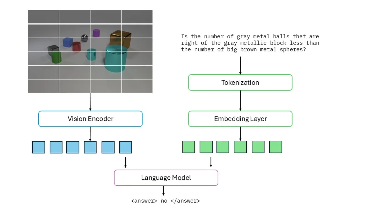
In LLMs, text is tokenized into a sequence of tokens, which are then converted into semantic vector representations, or embeddings, using an embedding layer. A similar process is applied to images. Instead of tokenizing text, images are divided into patches, encoded into embeddings by a vision encoder, and then aligned with text token embeddings. These image embeddings are then treated similarly to text embeddings when processed by the model.

For example, given a 64 × 64 image, we can divide it into four 16 × 16 patches (assume patch_size is 16) . Each patch is projected into an embedding space and then concatenated with text embeddings before being processed by the LLM. The processed is illustrated by the following figure:

Combining a Vision Encoder with an LLM

To accelerate experimentation, rather than training a vision encoder from scratch, we can take a pre-trained vision encoder and a base LLM and combine them. The Qwen-VL series has demonstrated strong performance on vision-language tasks, making it an ideal choice. In this experiment, we will use the vision encoder from a Qwen 2.5-VL 3B model and pair it with the Qwen 2.5 0.5B language model, which is lightweight enough to run on a single consumer-grade GPU. For implementation details on how these two models are integrated, refer to the notebook linked here. You can find the integrated model on huggingface.

Task: Visual Counting

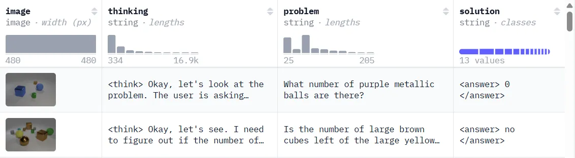
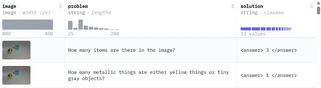
To keep the experiment simple, we will focus on an visual counting task, similar to the one in Deep-Agent/R1-V. The dataset Clevr_CoGenT_TrainA_R1, which contains around 37.8k data of image, question, reasoning trace like R1 and final answer. It consist of images such as:

Let's see how the model perform before training. Given the image below, and the prompt as How many items in the image?

Below is the response generated from the custom model. Which...doesn't make sense at all.
Let's see if we can improve it with SFT.

Stage 1: Supervised Fine-Tuning (SFT)

Using pure GRPO to fine-tune the custom VLM is difficult because the rewards are too sparse and the internal representations of the LLM were never tuned for visual information. The learning signal are just not too strong enough to guide the model. In fact, even DeepSeek R1 use SFT as a warmup stage before perform the GRPO! Therefore, we will first perform SFT on dataset shown previously.

Let's walk through some major code on SFT.

Model Loading

In this setup, we freeze most of the model’s weights, except for the last layer of the vision encoder, embedding layer and the first five layers of the language model. The rationale behind this is that both the vision encoder and language model have already been well-trained in their respective domains, and we want to preserve their learned representations. Instead of significantly altering their original weights, we focus on aligning visual information so that the language model can process image tokens in a way similar to text tokens. We set the max_pixels (the max pixels of the image to resize the image.) to 256 * 256 to keep it small but still visible to reduce the image tokens and overall computation.

max_pixels = 256 * 256
processor = AutoProcessor.from_pretrained(
    model_name, max_pixels=max_pixels, use_cache=False
)

model = Qwen2_5_VLForConditionalGeneration.from_pretrained(
    model_name,
    torch_dtype=torch.bfloat16,
    device_map="cuda",
    attn_implementation="flash_attention_2", # reduce memory usage and faster attention
    use_cache=False,
).to("cuda")

processor.tokenizer.padding_side = "left"

for param in model.parameters():
    param.requires_grad = False
  
for layer in model.model.layers[:5]:
    for param in layer.parameters():
        param.requires_grad = True

for name, param in model.visual.named_parameters():
    if "merger.mlp.2" in name:
        param.requires_grad = True
    else:
        param.requires_grad = False

Dataset processing

Next, we will download the data and prepare it by perform some formatting. We will split the dataset into 90% training and 10% for validation.

def is_valid_image(image_dict):
    """
    Given an image dictionary (with raw bytes), try to open the image.
    Returns True if the image can be successfully loaded; otherwise, False.
    """
    image_bytes = image_dict.get("bytes")
    try:
        img = PILImage.open(BytesIO(image_bytes))
        img.load()
        return True

    except (UnidentifiedImageError, Exception) as e:
        print("Skipping image due to error:", e)
        return False

def format_data(sample):
    image_dict = sample["image"]
    pil_image = PILImage.open(BytesIO(image_dict["bytes"]))
    pil_image.load()
    return [
        {
            "role": "system",
            "content": [{"type": "text", "text": SYSTEM_PROMPT}],
        },
        {
            "role": "user",
            "content": [
                {
                    "type": "image",
                    "image": pil_image,
                },
                {
                    "type": "text",
                    "text": sample["problem"],
                },
            ],
        },
        {
            "role": "assistant",
            "content": [
                {"type": "text", "text": f"{sample['thinking']}\n{sample['solution']}"}
            ],
        },
    ]


def get_data() -> Dataset:
    train_data, val_data = load_dataset(
        "MMInstruction/Clevr_CoGenT_TrainA_R1", split=["train[:90%]", "train[90%:]"]
    )
    train_data = train_data.cast_column("image", Image(decode=False))
    val_data = val_data.cast_column("image", Image(decode=False))

    return train_data, val_data


train_dataset, eval_dataset = get_data()
valid_train_dataset = [
    sample for sample in train_dataset if is_valid_image(sample["image"])
]
valid_eval_dataset = [
    sample for sample in eval_dataset if is_valid_image(sample["image"])
]
train_dataset = [format_data(example) for example in valid_train_dataset]
eval_dataset = [format_data(example) for example in valid_eval_dataset]

Custom data collator

We will define a custom data collator to process the data into batch. Note that we mask the prompt to train on completion only. You may remove that part if you wish to train on prompt as well.

# Create a data collator to encode text and image pairs
def collate_fn(examples):
    texts = [
        processor.apply_chat_template(example, tokenize=False) for example in examples
    ]
    image_inputs = [process_vision_info(example)[0] for example in examples]

    batch = processor(
        text=texts, images=image_inputs, return_tensors="pt", padding=True
    )
    labels = batch["input_ids"].clone()
    labels[
        labels == processor.tokenizer.pad_token_id
    ] = -100  # Mask padding tokens in labels

    # Ignore the image token index in the loss computation (model specific)
    if isinstance(
        processor, Qwen2_5_VLProcessor
    ):  # Check if the processor is Qwen2VLProcessor
        image_tokens = [
            151652,
            151653,
            151655,
        ]  # Specific image token IDs for Qwen2VLProcessor
    else:
        image_tokens = [
            processor.tokenizer.convert_tokens_to_ids(processor.image_token)
        ]  # Convert image token to ID

    # Mask image token IDs in the labels
    for image_token_id in image_tokens:
        labels[labels == image_token_id] = -100  # Mask image token IDs in labels

    answer_delimiter = "assistant\n"

    # Process each example individually to mask the question part
    for i, text in enumerate(texts):
        # Find where the answer starts in the raw text
        delimiter_index = text.find(answer_delimiter)
        if delimiter_index == -1:
            continue

        # Tokenize the portion of the text that comes before the answer.
        question_text = text[: delimiter_index + len(answer_delimiter)]
        question_token_ids = processor.tokenizer.encode(
            question_text, add_special_tokens=False
        )
        question_length = len(question_token_ids)

        # Set the corresponding tokens in the labels to -100 so that the loss is not computed on them.
        labels[i, :question_length] = -100

    batch["labels"] = labels
    return batch

Run training

Lastly, we define the SFTConfig and run the training!

# Configure training arguments
training_args = SFTConfig(
    output_dir=output_dir,  # Directory to save the model
    num_train_epochs=3,
    per_device_train_batch_size=1,  # Batch size for training
    per_device_eval_batch_size=2,  # Batch size for evaluation
    gradient_accumulation_steps=8,  # Steps to accumulate gradients
    gradient_checkpointing=True,  # Enable gradient checkpointing for memory efficiency
    # Optimizer and scheduler settings
    optim="adamw_torch_fused",  # Optimizer type
    learning_rate=2e-4,  # Learning rate for training
    lr_scheduler_type="cosine",  # Type of learning rate scheduler
    # Logging and evaluation
    logging_steps=10,  # Steps interval for logging
    eval_steps=5000,  # Steps interval for evaluation
    eval_strategy="steps",  # Strategy for evaluation
    save_strategy="steps",  # Strategy for saving the model
    save_steps=500,  # Steps interval for saving
    metric_for_best_model="eval_loss",  # Metric to evaluate the best model
    greater_is_better=False,  # Whether higher metric values are better
    # Mixed precision and gradient settings
    bf16=True,  # Use bfloat16 precision
    tf32=True,  # Use TensorFloat-32 precision
    max_grad_norm=0.3,  # Maximum norm for gradient clipping
    warmup_ratio=0.03,  # Ratio of total steps for warmup
    # Hub and reporting
    push_to_hub=False,
    report_to="mlflow",
    # Gradient checkpointing settings
    gradient_checkpointing_kwargs={
        "use_reentrant": False
    },  # Options for gradient checkpointing
    # Dataset configuration
    dataset_text_field="",  # Text field in dataset
    dataset_kwargs={"skip_prepare_dataset": True},  # Additional dataset options
    max_seq_length=2048,  # Maximum sequence length for input
)

training_args.remove_unused_columns = (
    False  # Keep unused columns in dataset since we might use it later
)

trainer = SFTTrainer(
    model=model,
    args=training_args,
    train_dataset=train_dataset,
    eval_dataset=eval_dataset,
    data_collator=collate_fn,
    tokenizer=processor.tokenizer,
)

trainer.train()

Evaluation

We will evaluate the model on out of distribution dataset (SuperCLEVR), which look a lot different than the training dataset! An example of sample from the evaluation set.
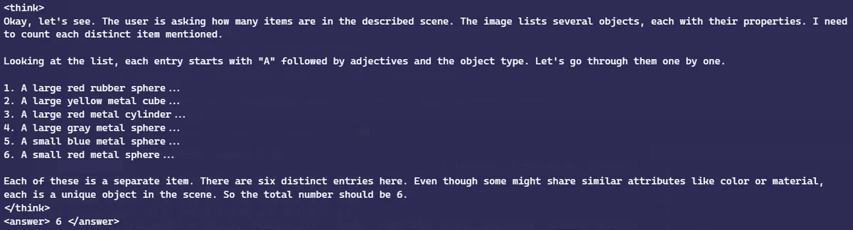
And our model after SFT can score around 68%! Here is the response generated by the model after SFT for the same previously tested image and question. Seems that it got it correct! Although the attribute of the object might be off, since we actually test on OOD images, which look completely different from training.

Stage 2: GRPO Fine-Tuning

TBH, fine-tuning with GRPO is a lot similar to SFT due to the abstraction provided by trl. The dataset we will use here is a similar dataset to our SFT stage, with difference in the absent of reasoning trace, which is Clevr_CoGenT_TrainA_70K_Complex. Now, the dataset contains only image, question and answer.
Our goal is to optimize for the solution while allowing the model to refine its reasoning on its own.

Define Reward Function

Since GRPO focuses on maximizing rewards, we need to define appropriate reward functions. We will primarily use the same reward functions as others work, specifically focusing on correctness and formatting. However, we may consider removing the format-based reward function, as the SFT stage already ensures that the model generates outputs in the correct format.

## Format reward
def detect_format(text: str) -> bool:
    pattern = r"^<think>([\s\S]*?)</think>\n<answer>([\s\S]*?)</answer>$"
    return re.fullmatch(pattern, text) is not None

## Reward functions
def correctness_reward_func(prompts, completions, answer, **kwargs) -> list[float]:
    responses = [completion[0]["content"] for completion in completions]
    q = prompts[0][-1]["content"]
    extracted_responses = [extract_xml_answer(r) for r in responses]
    log_dir = os.path.dirname(LOG_FILE)
    if log_dir and not os.path.exists(log_dir):
        os.makedirs(log_dir)

    with open(LOG_FILE, "a", encoding="utf-8") as f:
        f.write("-" * 20 + "\n")
        f.write(f"Question:\n{q[1]['text']}\n")
        f.write(f"Answer:\n{extract_xml_answer(answer[0]['content'][0]['text'])}\n")
        f.write(f"Response:\n{responses[0]}\n")
        f.write(f"Extracted:\n{extracted_responses[0]}\n")
    reward = [
        2.0 if r == extract_xml_answer(a["content"][0]["text"]) else 0.0
        for r, a in zip(extracted_responses, answer)
    ]
    with open(LOG_FILE, "a", encoding="utf-8") as f:
        f.write(f"Correctness reward: {reward}\n\n")
    return reward


def strict_format_reward_func(completions, **kwargs) -> list[float]:
    """Reward function that checks if the completion has a specific format."""
    responses = [completion[0]["content"] for completion in completions]
    matches = [detect_format(r) for r in responses]
    reward = [0.5 if match else 0.0 for match in matches]
    print(f"Strict format reward: {reward}")
    return reward

Customize GRPO Trainer

We cannot directly use the GRPOTrainer from Transformers 4.49 because it does not seem to support vision inputs. Therefore, we need to make some modifications by subclassing GRPOTrainer. Specifically, we will modify the compute_loss function to better fit our requirements. Additionally, we will remove code related to vLLM from the original GRPOTrainer for simplicity, although using vLLM could speed up training.
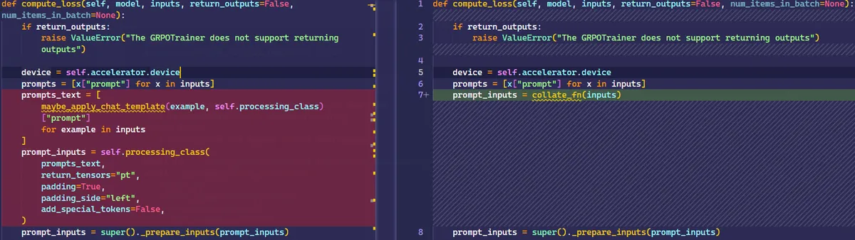
Second modifications would be remove the num_logits_to_keep arguments since Qwen 2.5 VL doesn't seems to support it.
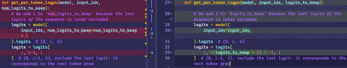
The rest of the function mostly remains the same.

Run training

Lastly, we define the GRPOConfig and run the training!

training_args = GRPOConfig(
    output_dir=output_dir,
    run_name=run_name,
    learning_rate=1e-5,
    adam_beta1=0.9,
    adam_beta2=0.99,
    beta=0.06,
    weight_decay=0.1,
    lr_scheduler_type="constant",
    warmup_ratio=0.05,
    logging_steps=1,
    bf16=True,
    per_device_train_batch_size=1,
    gradient_accumulation_steps=4,
    num_generations=8,
    max_prompt_length=None,
    max_completion_length=500,
    num_train_epochs=2,
    save_steps=50,
    max_grad_norm=0.1,
    log_on_each_node=False,
    use_vllm=False,
    report_to="mlflow",
)

trainer = VLGRPOTrainer(
    model=model,
    processing_class=tokenizer,
    reward_funcs=[strict_format_reward_func, correctness_reward_func],
    args=training_args,
    train_dataset=train_dataset,
)

trainer.train()

I train it for around 600 steps and evaluated the model on the OOD dataset again and achieved a 73% accuracy! While the performance gain isn't massive, it's still a solid +5% improvement. Considering that we started with a custom model with no prior visual training, reaching a 73% score on visual counting is a significant achievement!

Final Remark

In this blog, we dive into the math behind the GRPO equation, which has played a key role in improving the reasoning abilities of DeepSeek Zero and R1. We also explore how to fine-tune a language model with no prior visual training into one that can actually perform visual counting.

One interesting takeaway: keeping the learning rate around 1e-5 and constant seems to work best for GRPO in this case. I actually tried fine-tuning a custom model purely with GRPO, but it didn’t work out. However, when I used a well-trained VLM as a reference model, cranked up the beta parameter (which controls KL) really high, and trained for about 50 epochs, the model did pick up some visual concepts. The results weren’t amazing, though, and the whole process was just way too expensive to be practical—at least for now. But hey, it was a fun experiment!

Feel free to explore various hyperparameters and reward functions to see what works best.

Thank you for reading!

#llm #paper-reading #rl