FlashAttention: Fast and Memory Efficient Exact Attention with IO Awareness

Transformers

Ever tried naming a Large Language Model (LLM) that doesn’t have a Transformer hiding under its hood? I’d bet you’d have an easier time getting a cat to walk on a leash without transforming into a furry tornado of chaos. The ubiquity of Transformers in this field isn’t mere coincidence, but they have reshaped the landscape of natural language processing due to their ability to contextual understanding, handling of long-range ddependencies, parallel computation..etc. As we all know, transformers architecture mainly consist of a encoder and decoder where encoder processes the input data (say, a sentence in English), and the decoder takes this processed input and transforms it into the desired output (like a translated sentence in French). Now, what sets Transformers apart is their pièce de résistance - the ‘attention mechanism’, which are also the critical component that fundamentally drives both the encoder and decoder.

Attention

The attention mechanism, an integral component of Transformer models, is a mathematical method that directs the model’s focus towards the most relevant parts of the input data. In the realm of natural language processing, the attention mechanism assigns different ‘importance’ levels to different words in a sentence. For instance, in the sentence “The cat, which we adopted last week, loves to play with yarn”, more ‘attention’ may be given to the words “cat” and “play,” while words such as “which” or “the” may be deemed less significant.

A specific form of attention, known as ‘self-attention’, takes this concept a step further in the context of Transformers. In self-attention, a sentence is processed word by word, with each word checking out every other word to determine how much it should influence the output. This influence is calculated using Query (Q), Key (K), and Value (V) vectors. Here’s a little glimpse into the math behind it:

For each word, we create a Query, a Key, and a Value vector.
We then calculate the dot product of the Query vector of the word we are focusing on (let’s call it Word A) with the Key vector of another word (let’s call it Word B).
This gives us a score, indicating how much Word B should influence Word A.
We repeat this for all words in the sentence, getting a bunch of scores. We then apply a softmax to these scores, which makes them sum up to 1. These softmax scores are our ‘attention’ scores.
Finally, we multiply the attention scores with their corresponding Value vectors and sum them up to get the output for Word A.

import torch
import torch.nn.functional as F

def self_attention(query, key, value):
    # Step 2: Compute dot product between Query and Key
    attention_scores = torch.bmm(query, key.transpose(1, 2))

    # Step 4: Apply softmax to the attention scores
    attention_scores = F.softmax(attention_scores, dim=-1)

    # Step 5: Multiply scores with Value vectors and sum them up
    output = torch.bmm(attention_scores, value)

    return output, attention_scores

# Create an example batch of word embeddings 
# (B = batch size, T = number of words, D = embedding size)
B, T, D = 10, 5, 100
embeddings = torch.rand(B, T, D)

# Step 1: Create Query, Key, Value for each word
query = key = value = embeddings

output, attention_scores = self_attention(query, key, value)

print("Output shape: ", output.shape)  # Expected: [B, T, D]
print("Attention scores shape: ", attention_scores.shape)  # Expected: [B, T, T]

Notes: this is a simplified demonstration of the self-attention process. In actual transformer models, the query, key, and value vectors are not the same and are generated from the input embeddings through separate linear transformations.

What is the problem with self-attention?

Despite its considerable benefits, self-attention isn’t without its shortcomings. The central challenge lies in its inherent computational complexity when handling long sequences. For a sequence of length ‘n’, the time and memory complexity of self-attention scales quadratically with ‘n’, since each token or word in the sequence needs to attend to every other token, resulting in $n^2$ connections. A considerable amount of research has been directed towards minimizing the computational and memory prerequisites of attention, yet improvements in wall clock speed are often minimal. The reason is that they tends to focus on floating point operations (FLOPs) reduction (which may not correlate with real-time speed) and tend to ignore overheads from memory access (IO). Furthermore, these methods often approximate standard attention, meaning that their output values are not exactly identical to those yielded by standard attention. Before we discuss further, let’s understand the architecture of GPU:

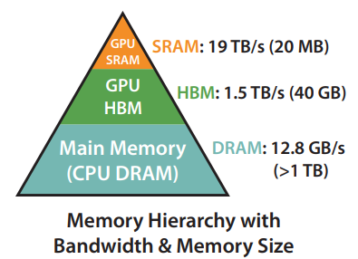
The figure above illustrates the structure of the GPU memory hierarchy. At the base of this hierarchy, we find the CPU DRAM followed by the GPU’s High Bandwidth Memory (HBM) and then the GPU’s SRAM at the top. In the context of deep learning computations, the data is predominantly stored in HBM, owing to its larger storage capacity (40-80GB for the A100 GPU). However, due to SRAM’s superior bandwidth (a whopping 19TB/s compared to HBM’s 1.5-2.0TB/s), data needed for immediate computations is loaded (Read) into SRAM. This places the data in closer proximity to the processing cores that execute the calculations. Once processed, the data is transferred back (Written) from SRAM to the more capacious HBM for storage.

Now, let’s understand another two important concepts.

Compute-bound: When the time accessing HBM is smaller than time taken to perform arithmetic operations, then compute time becomes matter. Memory-bound: When the compute has gotten faster relative to memory speed, then memory operations are increasingly bottlenecked by memory (HBM) accesses. Thus exploiting fast SRAM becomes more important.

According to the experiments conducted by the paper’s authors, it appears that the attention mechanism in Transformers is bottlenecked by the memory-bound issue. The figure above show this by highlighting that even straightforward operations like dropout, softmax, or masking consume more time compared to matrix multiplication. This increased duration is attributed to the read and write operations involved in moving the large $n * n$ attention matrix to HBM. In essence, these operations of transferring the attention matrix between HBM and SRAM appear to be the restrictive factor slowing the overall speed of attention computations.

Flash Attention

Based on the observations, they suggest that avoid reading and writing the attention matrix to and from HBM is essential to improve the wall-clock speed of attention mechanism. To reduce the read and write operations, they can:

Carrying out the softmax reduction in blocks (since reading and writing the complete attention matrix is resource-intensive). This is addressed through the implementation of Tiling.
Avoid storing the large intermediate attention matrix for the backward pass, which is tackled using Recomputation.

They place a specific emphasis on the reduction of the softmax operation because computing softmax in a block-by-block manner poses a unique challenge compared to other operations like dropout or masking. This complexity is rooted in the fact that softmax operations demand the entire input for computations. To explain in details, let’s recap the softmax operations, given an input vector $x$ of length $n$, the softmax function outputs a probability distribution $p$, also of length $n$, where the sum of the probabilities are equal to 1. Here is the steps to calculate softmax:

Exponentiate each element in the vector x.
Sum up all the exponentiated elements. This is the denominator for the softmax equation.
For each element in x, the corresponding value in p is the exponentiated value of the element in x divided by the denominator you calculated in step 2. which can also be expressed as: $\begin{align*} & p_i = \frac{exp(x_i)}{Σ_j exp(x_j)} \end{align*}$ To avoid numerical stability (exponentiating large numbers can result in an overflow), a common trick is to subtract the maximum value in the input vector from every value in the vector before computing the softmax. $\begin{align*} & p_i = \frac{exp(x_i - max(x))}{Σ_j exp(x_j - max(x))} \end{align*}$

Therefore, it is clear that without the entire input, it is difficult to perform the softmax computations.

Tiling

Luckily, For vectors $x^{(1)}, x^{(2)} \in \mathbb{R}^B$, we can decompose the softmax of the concatenated $x=\left[x^{(1)} x^{(2)}\right] \in \mathbb{R}^{2 B}$ as: $\begin{align*} & m(x)=m\left(\left[x^{(1)} x^{(2)}\right]\right)=\max \left(m\left(x^{(1)}\right), m\left(x^{(2)}\right)\right), \\ & \quad f(x)=\left[\begin{array}{ll} e^{m\left(x^{(1)}\right)-m(x)} f\left(x^{(1)}\right) & e^{m\left(x^{(2)}\right)-m(x)} f\left(x^{(2)}\right) \end{array}\right], \\ & \ell(x)=\ell\left(\left[x^{(1)} x^{(2)}\right]\right)=e^{m\left(x^{(1)}\right)-m(x)} \ell\left(x^{(1)}\right)+e^{m\left(x^{(2)}\right)-m(x)} \ell\left(x^{(2)}\right), \\ & \quad \text { softmax }(x)=\frac{f(x)}{\ell(x)} \\ & \end{align*}$ Therefore, if we keep track of some extra statistics (𝑚(𝑥), ℓ(𝑥)), we can compute softmax one block at a time. Or more inuitively:

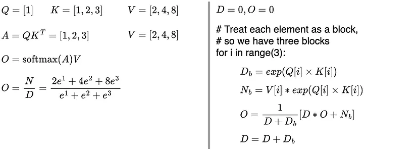
Figure 1. A Toy Q, K, and V matrixes to illustrate the difference between standard and flash attention. (Left) Standard attention computes and stores the entire attention matrix A to compute the attention output O; (Right) Flash attention operates on individual blocks of attention matrix A (A[i]=Q[i]*K[i]). So there is no need to compute and store the entire attention matrix A. Credit from Ahmed Taha

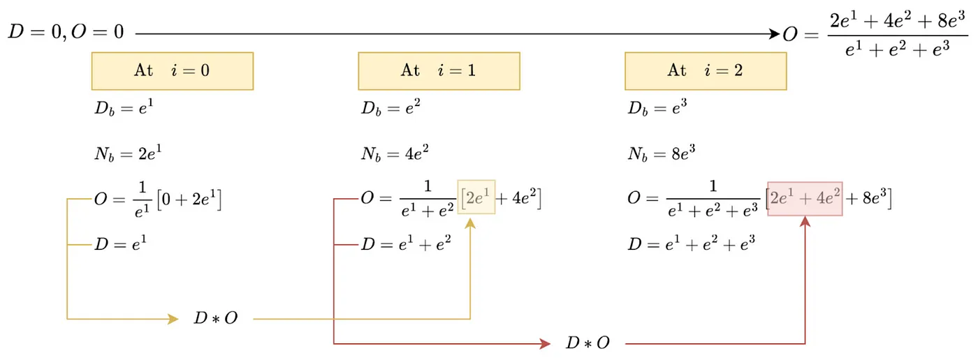
Figure 2. An illustration for the pseudo-code from Fig. 7 applied on the toy Q, K, V matrixes. Flash attention computes exact softmax operation using summary statistics {D, and O} and without storing the attention matrix A. The official flash attention uses more statistics (e.g., m=max(row)) for numerical stability. These extra statistics are omitted for presentation purposes. D_b denotes the current block denominator/numerator, while D is a summary statistic that tracks the row denominator. Credit from Ahmed Taha

Visualization from Francisco Massa

Recomputation

So, we now have a strategy for computing softmax (or other operations) in a block-by-block manner. However, we still have not figure out way to avoid storing the large intermediate attention matrix for the backward pass. But again, the $\mathbf{S}$ ($\mathbf{S}=\mathbf{Q K}^{\top}$), $\mathbf{P} \in \mathbb{R}^{N \times N}$ ($\mathbf{P}=\operatorname{softmax}(\mathbf{S})$) that required for backward pass can be easily compute from the previously stored (𝑚(𝑥), ℓ(𝑥)) and O (O=PV).

Although the proposed solution increase the FLOPs, but the overall wall-clock speed is still improved due to the reduced HBM accesses. The memory complexity also scaled down from quadratic $n^2$ to linear in sequence length.

Results

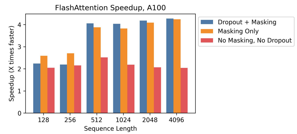
The figure presented below provides a comparative analysis of the speed enhancements over standard PyTorch attention across various sequence lengths, conducted on an A100. It can be seen that as the quantity of operations increases, the speed boost becomes more significant. This can be attributed to the process of kernel fusion, which combine multiple operations into a single operation.

Another exciting result is the training time of BERT-large, starting from the same initialization provided by the MLPerf benchmark, to reach the target accuracy of 72.0% on masked language modeling. Averaged over 10 runs on 8×A100 GPUs. Side note: the training time for huggingface implementations is 55.6+-3.9 minutes.

There are more results (also theoram proving) presented on the paper, which I highly recommend checking out to understand more about the details.

Conclusion

In conclusion, this paper presents a very interesting idea of tackling the computational complexity from the perspective of GPU hardware. Even though the proposed flash attention methods may initially seem to increase FLOPs, the overall impact is a net positive gain in wall-clock speed and a more linear memory complexity. Nonetheless, there are constraints to be addressed - for instance, the substantial engineering effort needed for implementation, due to the requirement for new CUDA kernel for each attention variant, and the potential lack of transferability across different GPU architectures. This means that, currently, high-level frameworks like PyTorch may not easily support this approach, at least to the extent of my current knowledge. Despite these limitations, this is a very excited work that can be applied to not just attention but other layer of deep learning architecture which suffered from memory-bound issue. This could ultimately enhance computational efficiency, thus lowering the barrier to entry for individuals keen on deep learning but limited by resource constraints.